P50 scan19: full dish scan, the best fit
sphere, surface errors.
11mar20
last update: 24apr20
Links
clipping
using xyz distances
xy
projection of points (.png)
xz
projection of points (.png)
fitting the data to a
sphere
Table of
coef
plots show the 10 iterations of each fit
(.ps) (.pdf) (21mar10
added histogram of errors)
Results of fit
do the weights make a difference?
Location of
points that were excluded by the 2 fits
xy image of points after 3 and 4
parameter fits (.png)
histogram of points after fits vs xy
radius (.ps) (.pdf)
Surface errors from Fit
residuals(scanner orientation)
Surface radial errors using 4 parameter fit
(.png)
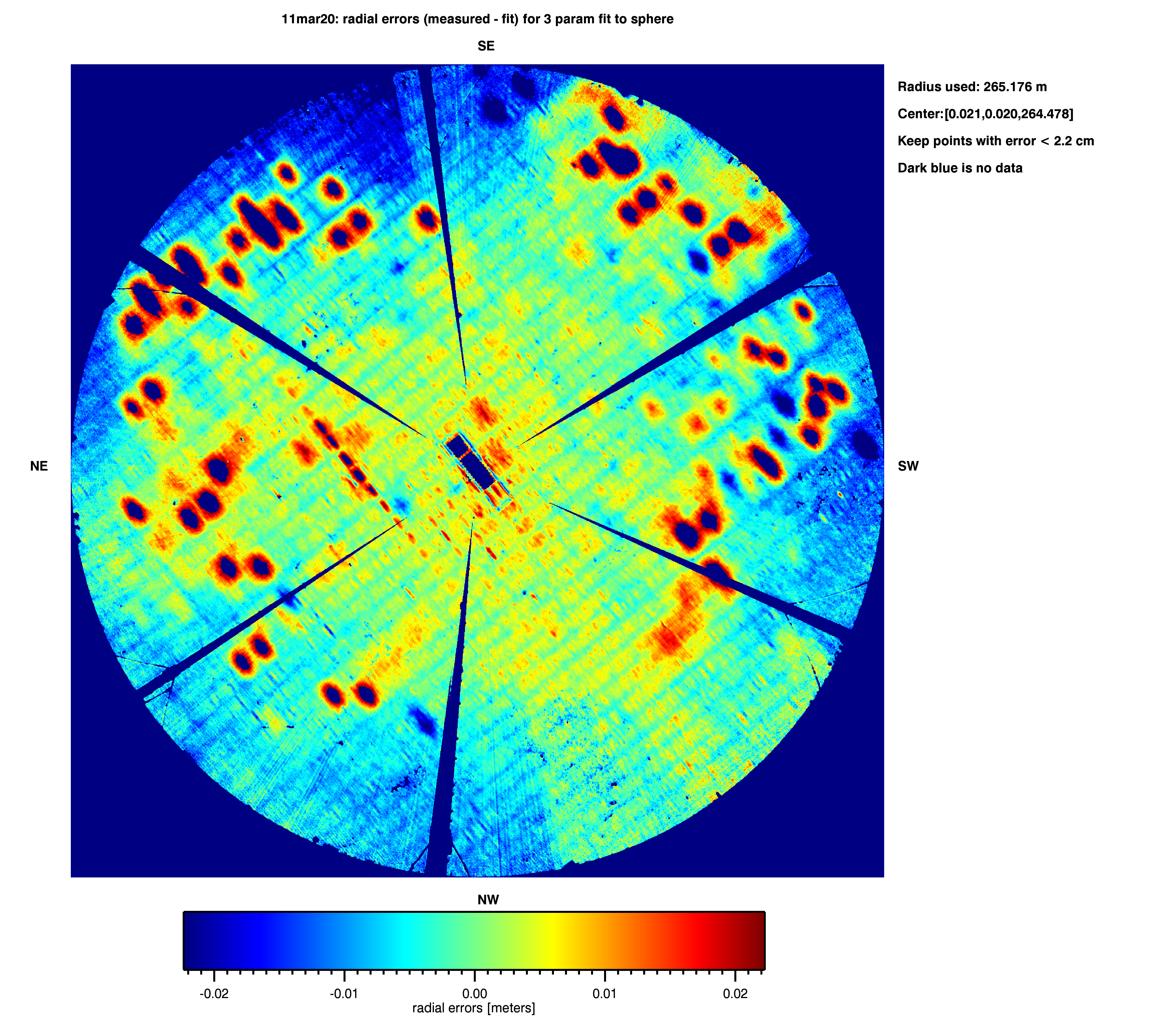
Surface radial errors using 3 parameter fit
(.png)
Surface
errors on the dish (n/s orientation) keep up to 5cm
radial surface errors < 5cm,
rotated to n/s orientation (.png)
Gain
loss from the surface errors
Summary
Other p50 pages
p50 main page
20200311 p50
scanning from ao9 main page
Facts:
- Design radius of curvature of primary for AO optics: 870
feet = 265.176 meters
Intro
Scan 19 was a full 360 degree scan of the dish
using 270 m ranging mode, high sensitivity, and 4mm spacing at
10m. It was used to fit a sphere to the data.
Two separate fits to a sphere were done:
- fit for the center and the radius of the sphere.
- Fit for just the center of the sphere. The radius was fixed at
265.176 meters (870 feet)
The main reason for the fits was to find the offset of the laser
scanner relative to the dish.
The 4 parameter fit (which included the radius) was
included:
- to try and get the best fit to the current curvature of the
dish (this is not necessarily the correct curvature for the AO
optics)
- When trying to average over area to reduce the measurement
error, we want to remove as much of the curvature as possible.
The scan was a complete 360 degree scan. We
only wanted to fit the part of the data that corresponded to
the dish so we clipped data by elevation range and xy radius.
There were still points that did not lie on the dish. To remove
them:
- Each fit was iterated 10 times
- on each iteration the rms was computed and then all
points with errors > 3 sigma were excluded for the next
iteration
- This actually excluded points that were part of dish.
Processing scan19
Scan 19 was the last scan taken. It start around
12:00 pm. It setup was:
- 270 m range mode
- full elevation -90 to 90 deg and full azimuth scan 0-360 deg.
It took about 27 minutes.
- So a large fraction of the scanned data is not on the dish
- There were 51297801 sampled points before any clipping.
- The scanner coordinate system was:
- y - points in direction where scanner started. In this case
it was about SE.
- x - points 90 east (cw looking down) from y. It was about SW
- z - perpendicular to x,y plane. Defined by the electronic
leveling of the p50 prior to start.
- Origin.
- the scanner was placed on the ao9 mount and then leveled
electronically.
- We did not use the laser pointer to translate the p50 to
be exactly over the ao9 monument
- the center for the scanner was about .7 meters above the
dish (I'm just eyeballing this).
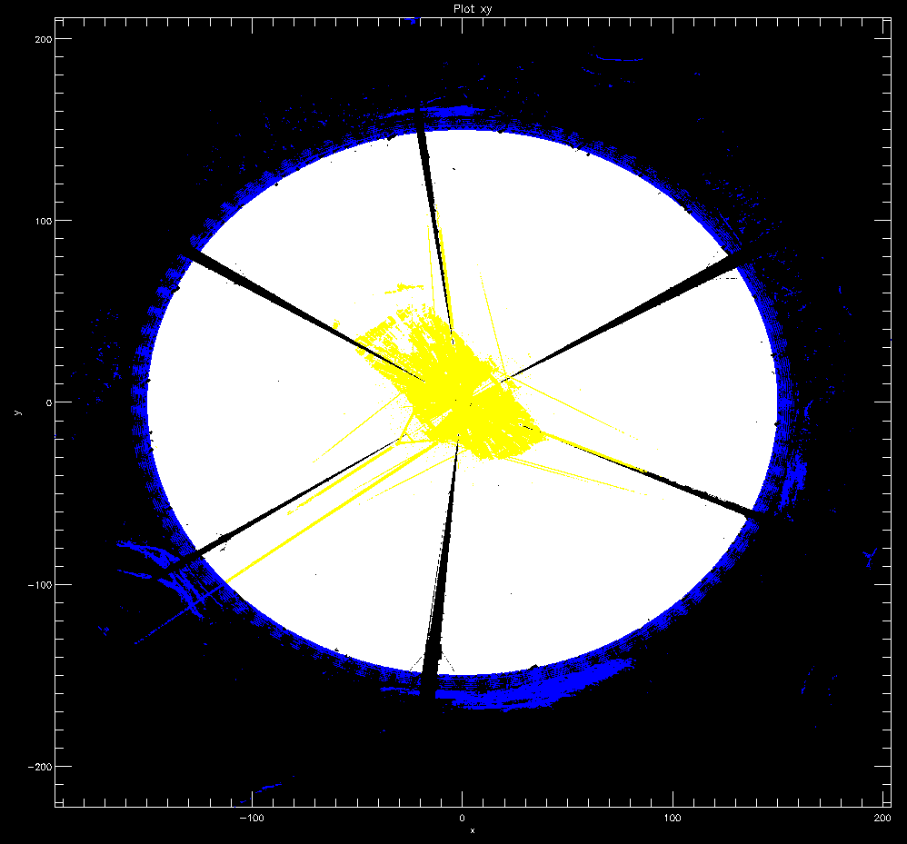
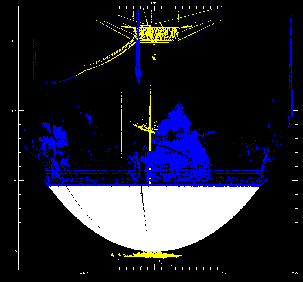
Clipping the
data use xyradius and elevation range.
The first round of clipping just used
geometrical distances to remove points not on the dish:
z range
|
-.7 to 47 meters
|
xy radius
|
150 meters
|
elevation range
|
-20 to 18 degrees
|
After clipping the points went from 51297801 to 16322830
The images show the xy and xz projections before and after
the clipping. colors were used to show why the points were clipped
- yellow - z limit clipping
- blue - xy radius clipping
xy projection of points (.png)
xz projection of points (.png)
Fitting a sphere to the clipped data.
- A sphere was fit to the 16.3 million points after
clipping. Two fits were attempted:
- 0= R0 - sqrt((x-X0)^2 + (y-Y0)^2 + (z-Z0)^2)
- fitting for R0,X0,Y0,Z0
- R0 is the radius
- X0,Y0,Z0 is the center of curvature of the sphere relative
to the scanner center (it is offset a bit from A09)
- 0=Rfixed - sqrt((x-X0)^2 + (y-Y0)^2 + (z-Z0)^2)
- Rfixed was set to 265.176 meters. This is the expected
radius (870ft) of the primary
- X0,Y0,Z0 were fit
- The areal density of points decreases as the distance
from the scanner increases.
- The points were weighted so the interior points (close to
the center) did not dominate the fit.
- A histogram in xy radius with 1 m binning was done.
- the number of points in a range bin were divided by the area
of the annulus to get the point density for this range bin.
- All xyz points within each range bin were then weighted by
1/sqrt(areaDensity).
- There were still many outliers in the 16.3 million pnts.
To get rid of them:
- The fit was iterated 10 times:
- After each iteration dR= Rmeasured - Rfit was computed for
each of the points in the fit and the weights were recomputed.
- Any points above 3 sigma were discarded, and the fit
continued looping.
- 10 iterations were probably more than we should have done,
but i wanted to see how things changed.
- I also wanted a good X0,Y0,Z0,R0 to use for future fitting
of other scans.
The plots show the 10 iterations of
each fit (.ps) (.pdf)
- Black lines are the 4 parameter fit for X0,Y0,Z0, and R0
- Read lines are the 3 parameter fit for X0,Y0,Z0 and R0 held
fixed at 265.176 m (870ft).
- Page 1: number of points and fit sigma
- Top: number of points at the start of each iteration
- The # of points in the fits started to diverge around the
5th iteration
- Bottom: Fit sigma for each iteration
- This was computed from measuredRadius - fitRadius
- The fit with constant radius started to diverge from the 3
parameter fit after iteration 5 (around 1cm rms).
- Page 2: fit coefficients for each iteration
- Top: X0 (+), Y0 (*) for the 20 iterations.
- X0 acted the same for both fit types
- Y0 tended more to 0 with the 4param fit.
- The coef for the last iteration are printed at the bottom
of this frame.
- Middle: Z0 coef for the iterations.
- This was stable for both types after the 3rd iteration
(1.2 cm sigma)
- Bottom: Radius for each iteration
- The red was fixed at 265.176
- Page 3: histogram of the radial errors.
- The histogram used 1mm bins. The errors came from the finale
iteration of each fit.
- Black is the 4 parameter fit, red is the 3 parameter with a
fixed radius.
- The errors for the 4 parameter fit is asymmetric with more
negative errors (the fit radius is longer than a larger
fraction of the points.
- The 3 parameter fits with fixed radius is offset in the
opposite direction.
The table below has the coef values
and sigmas for each iteration of the fits
coef/sigmas from 4 parameter fit
|
X0
(m) |
sigX
(m) |
Y0
(m) |
sigY
(m) |
Z0
(m) |
sigZ
(m) |
Radius
(m) |
sigRadius
(m) |
fitErr
(m) |
Npnts
(m) |
| 1 |
0.0232 |
0.0041 |
0.0170 |
0.0041 |
265.3739 |
0.0198 |
265.9683 |
0.0184 |
0.6441 |
16322830 |
| 2 |
0.0204 |
0.0041 |
0.0210 |
0.0041 |
264.4986 |
0.0192 |
265.1918 |
0.0179 |
0.1116 |
16021857 |
| 3 |
0.0205 |
0.0041 |
0.0209 |
0.0041 |
264.4083 |
0.0197 |
265.1117 |
0.0184 |
0.0178 |
15888141 |
| 4 |
0.0206 |
0.0041 |
0.0205 |
0.0041 |
264.4131 |
0.0197 |
265.1161 |
0.0184 |
0.0094 |
15714213 |
| 5 |
0.0210 |
0.0041 |
0.0193 |
0.0041 |
264.4095 |
0.0199 |
265.1124 |
0.0185 |
0.0074 |
15302483 |
| 6 |
0.0212 |
0.0041 |
0.0186 |
0.0041 |
264.4073 |
0.0200 |
265.1100 |
0.0186 |
0.0065 |
14960690 |
| 7 |
0.0212 |
0.0042 |
0.0182 |
0.0041 |
264.4059 |
0.0200 |
265.1086 |
0.0187 |
0.0060 |
14734489 |
| 8 |
0.0213 |
0.0042 |
0.0179 |
0.0042 |
264.4049 |
0.0201 |
265.1076 |
0.0187 |
0.0057 |
14597749 |
| 9 |
0.0212 |
0.0042 |
0.0178 |
0.0042 |
264.4044 |
0.0201 |
265.1070 |
0.0188 |
0.0056 |
14521312 |
| 10 |
0.0212 |
0.0042 |
0.0177 |
0.0042 |
264.4040 |
0.0202 |
265.1067 |
0.0188 |
0.0055 |
14479594 |
coef/sigmas from 3 parameter fit
(R0=265.176m)
|
X0
(m) |
sigX
(m) |
Y0
(m) |
sigY
(m) |
Z0
(m) |
sigZ
(m) |
Radius
(m) |
sigRadius
(m) |
fitErr
(m) |
Npnts
(m) |
| 1 |
0.0219 |
0.0041 |
0.0178 |
0.0041 |
264.5256 |
0.0011 |
265.1760 |
0.0000 |
0.6477 |
16322830 |
| 2 |
0.0204 |
0.0041 |
0.0210 |
0.0041 |
264.4814 |
0.0011 |
265.1760 |
0.0000 |
0.1083 |
16018940 |
| 3 |
0.0206 |
0.0041 |
0.0208 |
0.0041 |
264.4772 |
0.0011 |
265.1760 |
0.0000 |
0.0181 |
15885711 |
| 4 |
0.0208 |
0.0041 |
0.0205 |
0.0041 |
264.4773 |
0.0011 |
265.1760 |
0.0000 |
0.0103 |
15707567 |
| 5 |
0.0211 |
0.0041 |
0.0200 |
0.0041 |
264.4775 |
0.0011 |
265.1760 |
0.0000 |
0.0086 |
15359749 |
| 6 |
0.0212 |
0.0041 |
0.0200 |
0.0041 |
264.4777 |
0.0011 |
265.1760 |
0.0000 |
0.0080 |
15115956 |
| 7 |
0.0213 |
0.0041 |
0.0201 |
0.0041 |
264.4777 |
0.0011 |
265.1760 |
0.0000 |
0.0077 |
14980718 |
| 8 |
0.0213 |
0.0041 |
0.0202 |
0.0041 |
264.4777 |
0.0011 |
265.1760 |
0.0000 |
0.0075 |
14911581 |
| 9 |
0.0213 |
0.0041 |
0.0202 |
0.0041 |
264.4777 |
0.0011 |
265.1760 |
0.0000 |
0.0074 |
14877046 |
| 10 |
0.0213 |
0.0041 |
0.0202 |
0.0041 |
264.4777 |
0.0011 |
265.1760 |
0.0000 |
0.0074 |
14860694 |
Notes:
- Npnts is the number of points on input to the fit.
Results of fit:
-
Fit Coefs after final iteration
# params
in fit
|
X0
[m]
|
Y0
[m]
|
Z0
[m]
|
R0
[m]
|
#pnts
|
4
|
0.0212 |
0.0177 |
264.4040 |
265.1067 |
14457027
|
3 (R0 fixed)
|
0.0213 |
0.0202 |
264.4778 |
265.1760 |
14852776
|
-
-
Coef differences between fits
|
X0
[cm]
|
Y0
[cm]
|
Z0
[cm]
|
center Fit3-Fit4
|
.01
|
.25
|
7.38
|
R0 (Fit3-Fit4)
|
|
|
6.93
|
-
-
Height of scanner above dish
fit
|
R0 - Z0
[meters]
|
4 param fit
|
.70
|
3 param fit
|
.70
|
-
- The radii between the two fits differed by 7. cm.
- The 4 parameter fit was trying to compensate for errors in
the curvature of the dish by shortening the radius of
curvature.
- The center positions are consistent
- the x0 offset had no difference
- the y0 offset differed by 3mm
- the z0 offset differs by 7.4 cm
- but this was because the radius changed by 7.0cm
- taking this into account, the z0 of the centers were
within 5mm
- the (Radius - Z0) should give the height of the scanner above
the dish surface. In both fits we got .7 meters.
- The scanner mirror is 25 cm above it's base
- the tribrach mount was about 2cm (never measured it).
- So the top of the ao9 mount should be .43 meters above the
dish surface..
- We can check this by measuring the height of the ao9 top to
the ao9 dimple.
- lynn (2002) says that the dimple is at a radius of 883.125
feet.
Do the weights make a difference?
- The fits were run with and without weights.
- The table below shows the coefficients from the fits without
and with weights.
- the last column shows the difference WeightedCoef -
unwaitedCoef
- The 3 parameter fit did not change (with 2mm)
- the 4 parameter fit made the radius longer by 6mm and moved
z0 up by this amount.
- There were many more points close to the center.
- they did not dominate the fit since changing the center or
radius makes very little difference in the fit error.
- The points at the edges are affected much more by changes in
the center or radius.
Compare Fits with Weights and no Weights
[meters]
|
3
param fit
|
4param
fit
|
|
x0
|
y0
|
z0
|
r
|
x0
|
y0
|
z0
|
r
|
noWeights
|
.0213
|
.0212
|
264.4756
|
265.176
|
.0213
|
.0177
|
264.3974
|
265.1007
|
with Weights
|
.0213 |
.0202 |
264.4778 |
265.176 |
.0212 |
.0177 |
264.4040 |
265.1067 |
W-NoW
|
.0
|
-.001
|
.0022
|
-
|
-,0001
|
0
|
.0066
|
.006
|
the plot shows a histogram of the
points vs xy radius and the weights used (.ps) (.pdf)
- top: histogram of points after 4 param fit iterations vs
the xyRadial distance.
- the histogram is binned to 1 meter.
- bottom: the weights used for points in each histogram bin were
1/sqrt(densityOfPoints)
- the densityOfPoints was computed at
numberOfPointsInBin/binArea
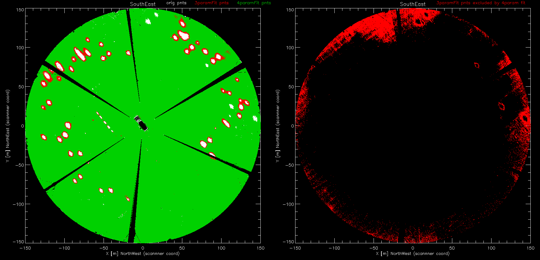
Location
of points that were excluded by the 2 fits
xy image of points after 3 and 4
parameter fits (.png)
- The image orientation can be seen from the black opening in
the middle of the dish.
- the upper left portion of the opening points east.
- For each fit all points > 3 sigma were excluded. This
iterated for the 10 loops.
- Left image: over plot, initial, 3param fit ,and 4 parameter
fit points
- The initial set of points used is plotted in white.
- The points kept after the 3 parameter fit are over
plotted in red.
- the points kept after the 4 parameter fit are over plotted
in green.
- points in white were remove by the 3 parameter fit
(3sigma=2.2 cm)
- points in red were additionally excluded by the 4
parameter fit (3sigma = 1.7cm)
- The black wedges are shadows cast by the hf
- the line of spots [-45,-10] to [-60,20] is the
east-west cable broken during hurricane maria
- The long hole at x=-100, y=90 is a panel that is bent up.
- Right image: points in fit3 excluded by fit4
- The red dots are points in fit3 that were excluded by fit4.
- We don't see this in the left image because there are not
enough pixels in the display.
Histogram of points after fit
exclusion (.ps) (.pdf)
- histograms were made of the numbers of points left after the
fit exclusion of points vs xyradius, azimuth, and elevation.
- black line: histogram of points before fit exclusion.
- red line: points after 3 parameter fit exclusion
- green line: points after 4 parameter fit exclusion.
- Top: histogram vs xy radial distance.
- the blue dashed line is the radial distance of the hf 8mhz
dipoles
- the purple dashed line is the radial distance of the hf 5
mhz dipoles.
- middle: histogram of points left after fit exclusion vs
scanner azimuth.
- azimuth 0 pointed SSE and increased CW.
- Blue dashed lines show the excluded points
around the 8 mhz hf dipoles
- the purple dashed lines show the excluded points around the
5 mhz dipoles
- The light blue dashed lines have excessive counts.The are
spaced by 180 degrees.
- since the scanner measures az and az+180 in one elevation
rotation, the scanner must have sat at this position for a
longer time?
- You can see a small variation in the number of counts vs
azimuth.
- If this was a scanner az rotation vel change, you would
expect a 180 periodicity. The variation is a little less
that 180 degrees and not exactly repeatable. It could just
be a variation in the azimuth velocity.
- Bottom: histogram vs elevation.
- since the scanner was about .7 meters above the dish, the
elevation can be < 0.
- we hit the edge of the dish when the elevation is a little
less than 18 degrees.
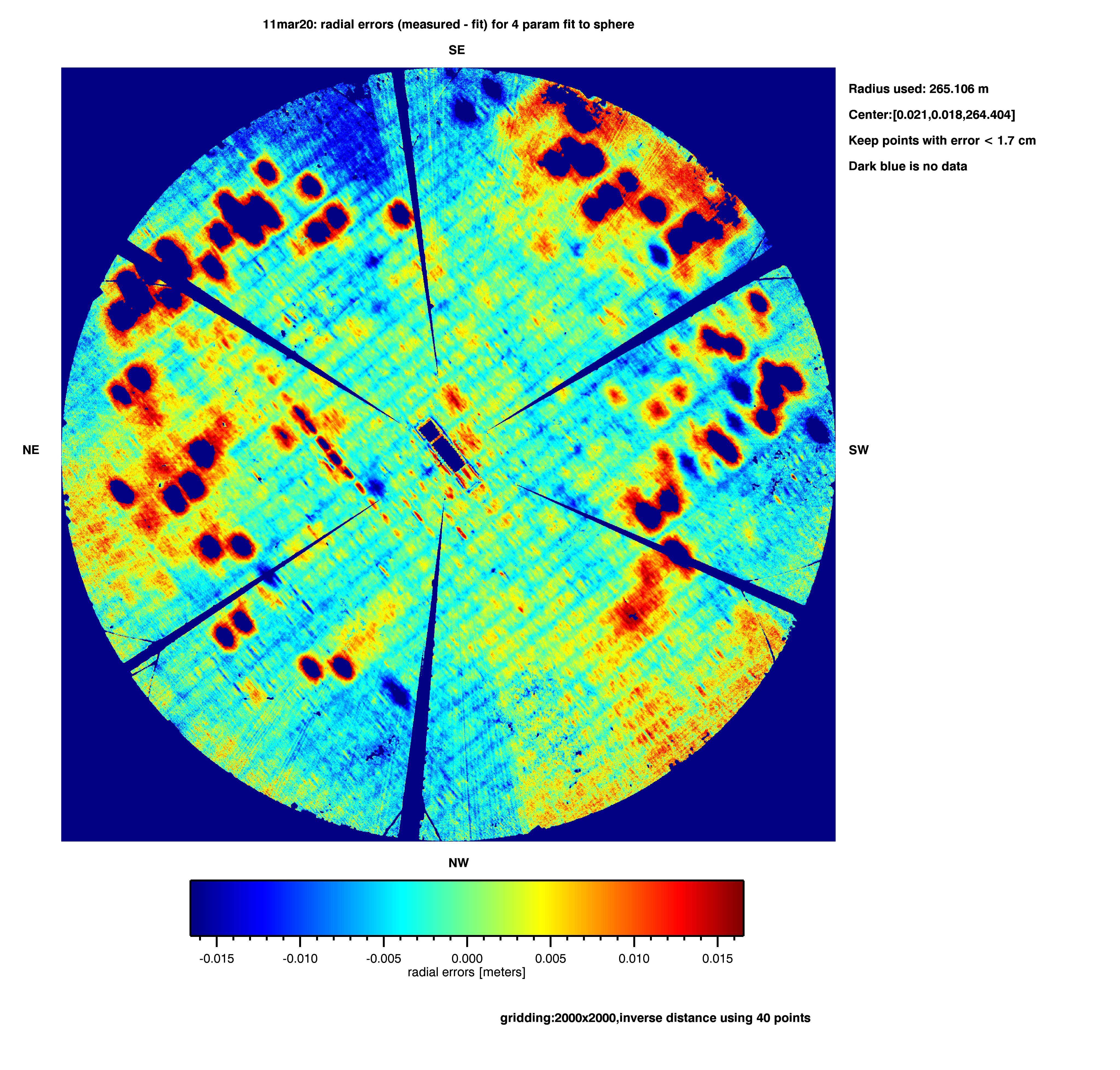
Surface errors
from using the fit residuals
The points that were left after iterating the
fits 10 times were used to make an image of the dish errors.
- All points with errors > 3 sigma from the last
iteration were excluded: (1.7cm , 2.1 cm)
- The x,y coordinate system was the scanner orientation.
- The x-y plane was gridded (2000,2000) points.
- this gave a resolution of 300M/2000= .15 meters
- the idl griddata routine was used with inverse distance
method, using only 40 points around each grid point.
Surface radial errors using 4 parameter
fit (.png)
Surface radial errors using 3 parameter
fit (.png)
- dark blue are points that were excluded from the fit because
their error was greater than the fit 3 sigma error.
- blue has (measured - fit) negative. So the points are
above the design surface.
- yellow ->red are positive so the points are below the
design.
- The diagonal stripes are spaced about 25 feet apart, so they
are probably the main cables
- This may be the flexing of the dish between the main cables
from heat expansion (we did this at noon).
- When the scanner hits a piece of the dish that sticks up, a
shadow will be created behind it.
- For the points in the shadow their measurement will place
them at the x,y location of the bent panel (but with a shorter
radius)
- So you should see a area turning blue and then no data (dark
blue).
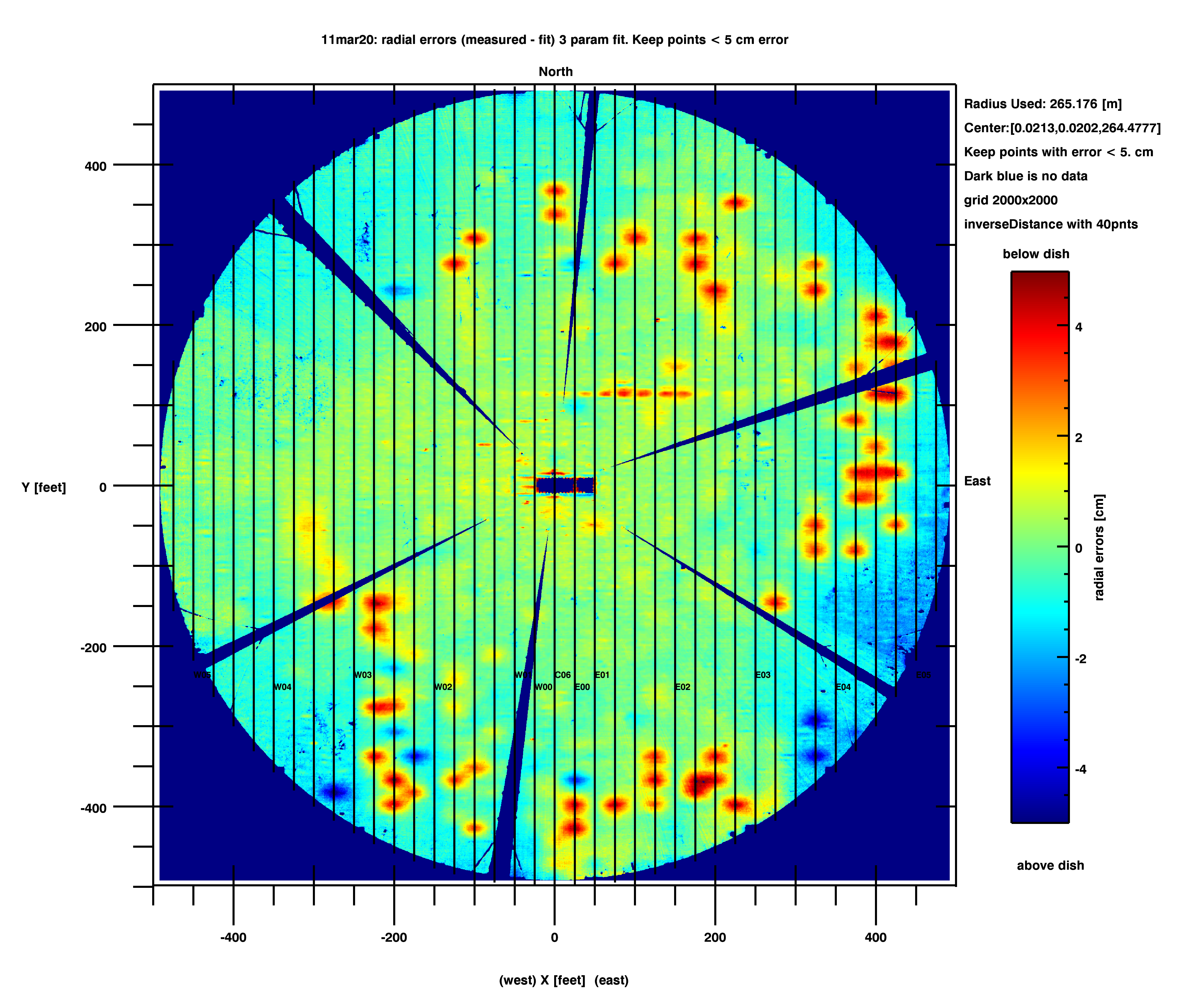
Surface errors using all points < 5cm
error
The radial error was computed for all
points using the 3 parameter fit center and the design radius of
265.176 meters.
- All points with radial error > 5cm were excluded
- The coordinate system was rotated to align with
north,south,east west.
- The point cloud data was displayed (using qtreader).
- The north/south row of panels could be seen. One of
these was chosen to measure their coordinates.
- The row that included the west edge of the missing
panels for td12 was used.
- the coord for the east and west edge of the panel row was
recorded for the northern, southern, and the location of the
missing panel
- a linear fit was done to get the slope of the line in the
scanner coordinate system.
- The slope of this line gave the angle between
the scanner x axis and the north south line of
the main cables: (39.26 deg CW +)
- rotating by 39.26 deg put the x axis of the scanner
aligned with south, another +90 degrees put the data aligned
with east
- the total angle was 129.26 ... i actually had to use
-129.26 in my routines since rotating a coord system
is the negative of rotating a vector.
- After rotation, the x,y coord were scaled to feet.
- All of the drawings are in feet, so it is easier to
reference locations on the dish in feet.
- the radial error was left in cm (since the wavelengths we
use are all in cm).
- The data was then gridded with idl's griddata routine.
- a 2000x2000 grid was used -> 300m/2000= .15 meter spacing
(sorry about jumping back and forth with units :)
- the inverse distance gridding was used. using the closest 40
points. If no points were available with .5 meters, the grid
points was marked as no data.
- An image was made using the iimage tool of idl.
- the blue->red color table covered -5cm to + 5cm (color
table is on the right side)
- vertical lines were placed at each of the main cables (25 ft
spacing).
- The cables were then labeled (i left out the a,b,c cables).
The image shows the surface
errors measured 11mar20 (.png)
- Any grid points with errors > abs(5cm) were excluded. They
are plotted in dark blue.
- Dark red is +5cm error.
- The error was computed as (MeasuredLength -design). A
positive value means the radius for that points is too long
(the point lies below the design surface).
- blue goes to -5cm. These points have a radius too short. The
point is above the design surface.
- The dark blue wedges are shadows cast by the hf dipoles:
- x=10.8,y=101 is the shadow from the 5mhz dipole in the
north. The other 5 mhz dipoles are spaced by 120 degrees.
- x=70,y=23 is the shadow from the 8 mhz dipole. It is larger
because it is closer to the scanner.
- Points of interest:
- x=335.2, y=-257.3.. this is a missing panel on the dish.
-
x
|
y
|
|
335.2
|
-257.3
|
this is a missing panel
|
-235.
|
304
|
dark blue area is vegetation growing on
the dish
|
100
|
114
|
- east-west cable broken during hurricane
maria.
- The new splice connected the e-w cable to the
adjacent mains
- The dark red shows the e-w cable was not pulled
tight enough and that it slipped between multiple
main cables.
- It is probably 3-4 cm low at the worst
spot.
- It spans about 11 main cables (275 feet)
|
160
|
-103
|
missing panels where td 4 goes through
the dish.
|
-112
|
0
|
- yellow between main cables (to low)
- but adjacent main cables are green (correct
height)
- This is probably the sagging of the main cables
caused by the temperature
- data was taken at noon on a cloudy but hot day
- The grid measurements showed the mean value of
the grid section moved by about 3mm in the 45
minutes of the 9 grid scans.
|
124
|
-337
|
- dark red ovals. These are also spread over much
of the dish, predominantly at the longer radii
(steeper slopes).
- They are all centered on the main cables..
- This is most likely the main cable tiedown cable
blocks have slid from their correct location.
|
processing: x101/p50/200311/doit.pro
The gain loss was computed using the measured
radial errors. The processing was:
- Use the 2000x2000 grid of radial surface errors. Any errors
> 5 cm were ignored (to remove things like hf dipoles)
- generate are 2k x 2k reference grid of random errors with an
rms of .22 cm. This was the goal for the 2000 survey results.
- Pick an x,y spot on the dish
- find all points with measured rms errors within 225/2.
meters of this point (beam radius)
- generate the phase errors for a particular wavelength for
these points: radialErrcm/lambdaCm * 2*pi.
- generate the complex E field for all of these points using
unity amplitude and the measured phase.
- Sum the E field for the reference and sum the Efield for the
measured points.
- Take the ratio of the intensities as the gain loss.
The plots show the gain loss results for
beams centered on a 5x5 grid with 200 foot spacing (.ps)
(.pdf)
- Each frame shows beams moving from -400 to +400 x
position. (- is west)
- The top frame is y = +400 (north), the bottom frame is -400 ft
(south)
- The gain loss was computed for 21, 12.3,6, and 3 cmd
(1420,2380,5000, 10000 Mhz)
- the colors show the different wavelengths
- The large errors at +x and -Y are mapping into gain
losses (especially at 10 ghz)
- The losses at x and cband are similar to what we see on the
telescope calibration runs.
- The sband losses are smaller than the ones we've measured on
the telescope.
- What these plots don't measure:
- I only took points on the dish.. for the measured and
reference beams. When the beam spilled over, i ignored those
points (since there were no measured errors). The plots do not
show the normal gain falloff because of the spillover.
- There may be points > 5cm that were excluded (by my
thresholding)
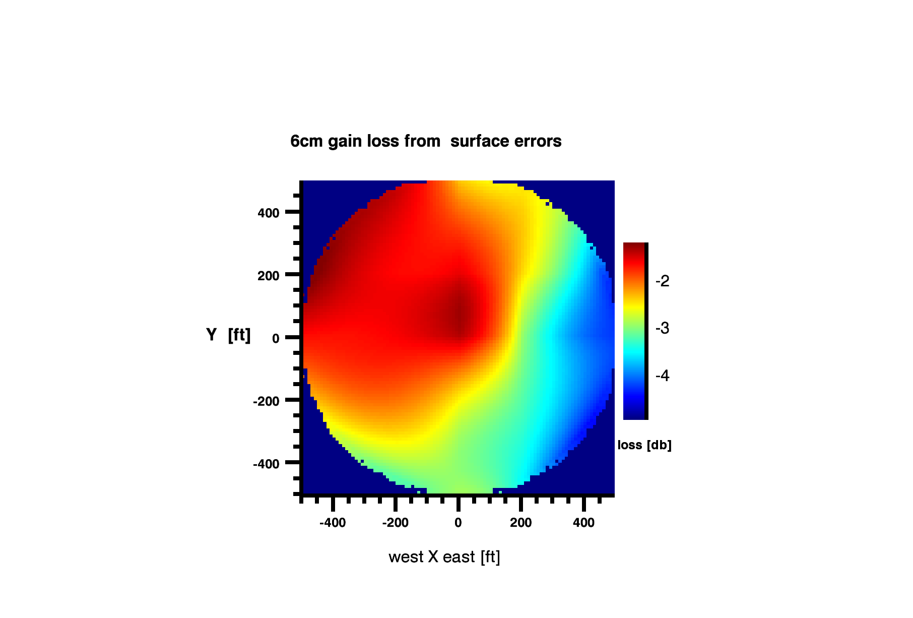
The image gives a rough idea of what
the gain loss should be at 6cm across the dish (.png)
- the image was made by creating a grid via interpolation
of the points in the line plot above.
processing: x101/p50/200311/gainloss.pro
Summary:
- scan19 had 16.3 million points that were used for a fit
to a sphere
- fitting 4 parameters (x0,y0,z0,r0) and 3 parameter
(x0,y0,z0,r0fixed). gave similar results
- x0,y0 was similar for both fits
- The z0 variation was correcting for the change in
radius
- So we can probably use the 3 parameter fit center and
radius and be good to maybe a cm or better.
- The value below can be used for any of the other scans
(since the p50 was not moved during the scans)
-
Center of curvature of dish in scanner coord.
Xcenter
[m]
|
Ycenter
[m]
|
Zcenter
[m]
|
Radius
[m]
|
.0213
|
.0202
|
264.4778
|
265.176
|
- After 10 iterations (throwing out 3sigma points after each
iteration) gave
- point reduction 16.3 to 14.6 million points
- fit sigma after 10 iterations: 5.5 mm, and 7.4 mm
- the fits were done with and without weighting the points (by
1/sqrt(arealdensity). it did not make much difference.
- residual images showed
- the sagging of the dish between the main cable
- The repaired east-west cable that was broken during maria
- the fits were for the best fit sphere. This is not
necessarily the correct location for the arecibo optics.
- We can use the 4 parameter best fit sphere to
remove the curvature when averaging over areas (see processing the wedges).
- Surface errors.
- After aligning the scanner azimuth with n/s and scaling to
feet an image was made of all points with < 5cm radial
error.
- We see a sagging between the main cables of up to a cm.
- the east-west cable that broke during hurricane maria
is mis adjusted by 3-4 cm. It's affect spans about 275 feet.
- there are numerous low spots (3-4 cm) centered on the main
cables.
- the cement blocks for the main cable tiedowns have
probably slipped.
- --> fixing the main cable tiedown blocks will probably
make a large improvement in the dish performance.
- We don't have to wait for the adjustment of all of the
panels.
processing: x101/p50/200311/fitsphere/fitsphere_fit.pro,
fitsphere_plt.pro,fitresidual_img.pro,
<- page up
home_~phil